[4]:
from pathlib import Path
from brainlit.utils.Neuron_trace import NeuronTrace
from brainlit.algorithms.trace_analysis.fit_spline import GeometricGraph
import numpy as np
import matplotlib.pyplot as plt
from matplotlib.cm import ScalarMappable
from mpl_toolkits.mplot3d import Axes3D
import matplotlib
from scipy.interpolate import splev
Fitting Splines to Neuron Trace SWC Tutorial
1) Define variables
swcthe geometric graphdf,_,_,_read the x, y, and z columns in swc fileneurondefine a new class inherited fromGeometricGraphclasssomadefine the data on the first run as the location of soma
[6]:
brainlit_path = Path.cwd().parent.parent.parent
swc = Path.joinpath(
    brainlit_path,
    "data",
    "data_octree",
    "consensus-swcs",
    "2018-08-01_G-002_consensus.swc",
)
nt = NeuronTrace(path=str(swc))
df = nt.get_df()
neuron = GeometricGraph(df=df)
soma = np.array([df.x[0], df.y[0], df.z[0]])
2) Plot the whole spline tree
spline_treeuse thefit_spline_tree_invariantto locate neuron branches
[8]:
fig = plt.figure()
ax = fig.add_subplot(111, projection="3d")
spline_tree = neuron.fit_spline_tree_invariant()
for node in spline_tree.nodes:
    path = spline_tree.nodes[node]["path"]
    locs = np.zeros((len(path), 3))
    for p, point in enumerate(path):
        locs[p, :] = neuron.nodes[point]["loc"]
    ax.scatter(
        locs[:, 0],
        locs[:, 1],
        locs[:, 2],
        marker=".",
        edgecolor="yellowgreen",
        linewidths=1,
        c="mediumblue",
        s=8,
    )
    ax.plot(
        locs[:, 0],
        locs[:, 1],
        locs[:, 2],
        linestyle="-",
        color="midnightblue",
        linewidth=0.8,
    )
ax.scatter(soma[0], soma[1], soma[2], c="darkorange", s=5)
ax.w_xaxis.set_pane_color((1.0, 1.0, 1.0, 1.0))
ax.w_yaxis.set_pane_color((1.0, 1.0, 1.0, 1.0))
ax.w_zaxis.set_pane_color((1.0, 1.0, 1.0, 1.0))
ax.grid(True)


plt.show()
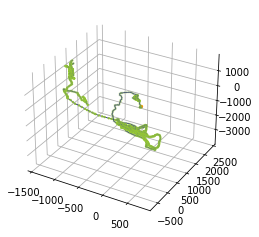
Figure 1. The green dots indicate the locations of nodes on a tree, representing a neuron, and the single orange dot locates the position of the soma. Each nodes are connected with darkblue lines to illustrate the path of the neuron.
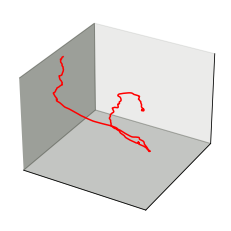
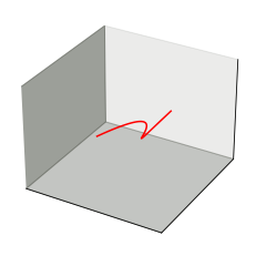
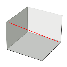
3) Plot each branch in separate plots
[9]:
for node in spline_tree.nodes:
    path = spline_tree.nodes[node]["path"]
    locs = np.zeros((len(path), 3))
    for p, point in enumerate(path):
        locs[p, :] = neuron.nodes[point]["loc"]

    spline = spline_tree.nodes[node]["spline"]
    u = spline[1]
    u = np.arange(u[0], u[-1] + 0.9, 1)
    tck = spline[0]
    pts = splev(u, tck)

    if node < 3:
        fig = plt.figure()
        ax = fig.add_subplot(111, projection="3d")
        ax.plot(pts[0], pts[1], pts[2], "red")
        ax.w_xaxis.set_pane_color((0.23, 0.25, 0.209, 0.5))
        ax.w_yaxis.set_pane_color((0.23, 0.25, 0.209, 0.1))
        ax.w_zaxis.set_pane_color((0.23, 0.25, 0.209, 0.3))
        ax.grid(False)
        ax.set_xticks([])
        ax.set_yticks([])
        ax.set_zticks([])
        plt.axis("on")
        plt.show()